Message passing in Gaussian Bayesian networks [3 P]

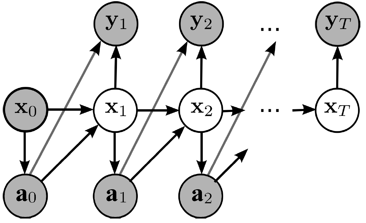
Consider the Bayesian network illustrated in Fig. 5 with the probabilities

$$P({\bf x}_0) = \mathcal{N}({\bf x}_0\vert{\bf a}_0,{\bf Q}_0)$$ (1)

$$P({\bf x}_{t+1}\vert{\bf x}_{t}) = \mathcal{N}({\bf x}_{t+1}\vert{\bf A}_t {\bf x}_{t} + {\bf a}_{t}\vert{\bf Q}_{t})$$ (2)

$$P({\bf y}_{t}\vert{\bf x}_{t}) = \mathcal{N}({\bf y}_{t}\vert{\bf D}_t {\bf x}_{t} + {\bf d}_{t}\vert{\bf C}_{t})$$ (3)

where $\mathcal{N}({\bf x}\vert{\bf\mu},{\bf\Sigma})$ denotes the multivariate Gaussian distribution with mean ${\bf\mu}$ and covariance $\bf\Sigma$ .

Figure: Gaussian Bayesian network.

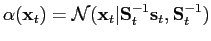
Prove that the forward messages have again the form of a Gaussian distribution

$$\alpha({\bf x}_t)=\mathcal{N}({\bf x}_t\vert{\bf S}_t^{-1}{\bf s}_t,{\bf S}_t^{-1})$$ (4)

with mean ${\bf S}_t^{-1}{\bf s}_t$ and covariance ${\bf S}_t^{-1}$ as defined on the slides for the exercise hour (slide 23). (Hint: Use the three properties of Gaussian distributions discussed in the exercise hour.)